Pipeline valve pressure drop calculation steps for system designers
A valve pressure-drop error propagates through the entire system. It distorts pump duty, reduces available control authority, increases actuator demand, and can move a liquid service into cavitation without any change to the P&ID.
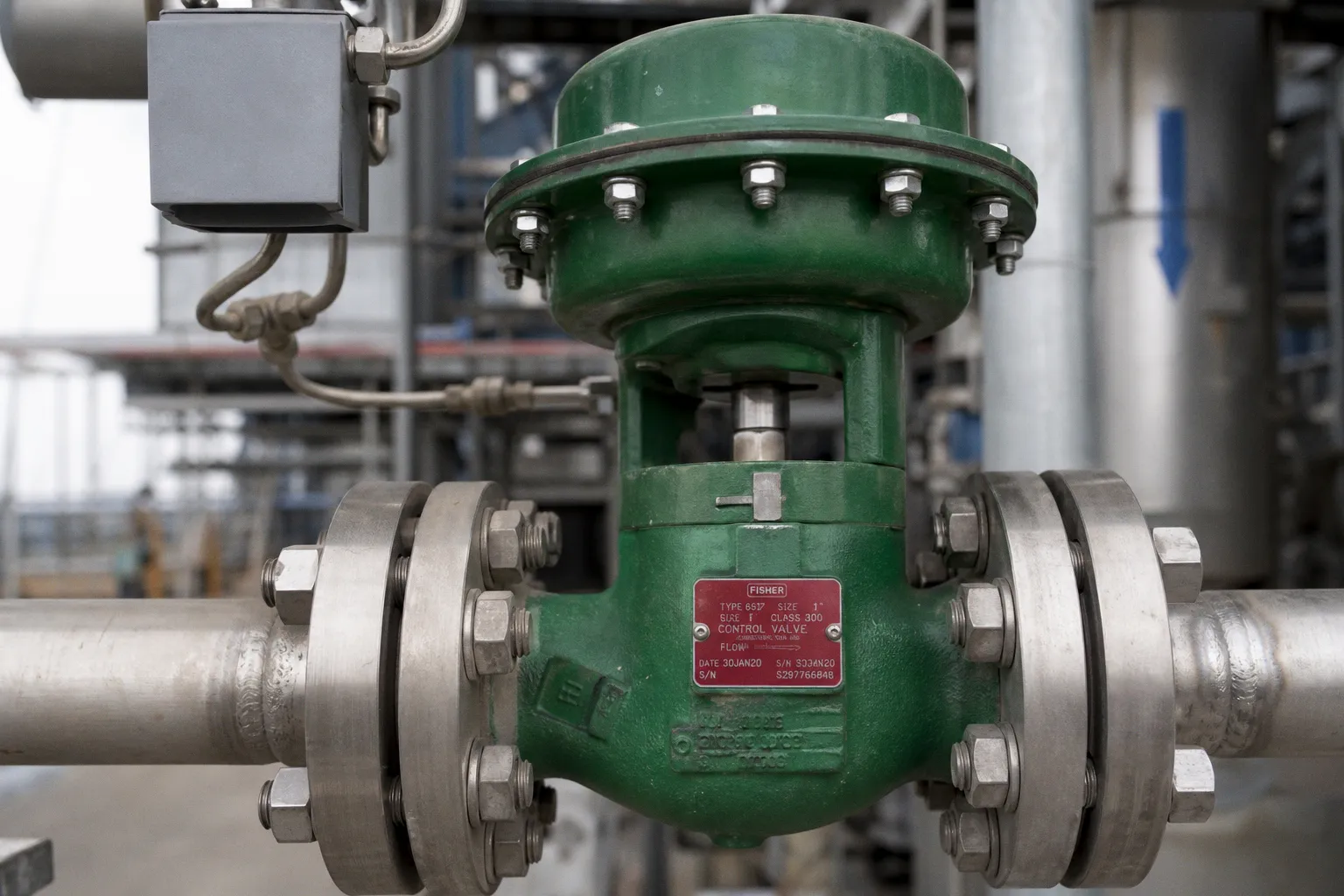
The usual cause is not a difficult equation. It is an invalid input model.
A pipeline valve pressure drop calculation method starts by classifying the valve’s role. A fully open isolation valve is usually treated as a fixed hydraulic resistance. A throttling control valve is a variable restriction and requires installed-capacity sizing. Gas and steam require compressible-flow treatment. Applying one method to all three cases produces a clean-looking result with a high error rate.
The calculation sequence should therefore be fixed before values are entered:
1. Define the design cases: minimum, normal, and maximum flow.
2. Capture fluid properties at operating temperature.
3. Establish actual internal pipe diameter and installed geometry.
4. Select the calculation model: loss coefficient \(K\), valve coefficient \(Cv\), or an IEC/ISA control-valve method.
5. Check the result against physical limits: choking, cavitation, flashing, compressibility, noise, and available pressure.
6. Recalculate after reducers, elbows, tees, or changes in valve trim are added to the installation.
The objective is not a single pressure-drop number. The objective is a pressure budget that remains valid at every operating point.
Start with the installed system, not the nominal valve size
Nominal pipe size is a catalog label. It is not a flow area, a valve capacity, or a pressure-loss result.
A DN100 or NPS 4 line can have different internal diameters depending on schedule, lining, corrosion allowance, and material. A full-port ball valve, reduced-port ball valve, globe valve, butterfly valve, and swing check valve of the same nominal size do not impose the same resistance. Their flow paths are different. Their recovery behavior is different. Their loss coefficients and \(Cv\) values are different.
The minimum dataset for a defensible calculation includes:
- Design, normal, and minimum flow rate. Use mass flow or volumetric flow consistently. For liquids, volumetric flow must correspond to the operating temperature.
- Fluid density at operating temperature. Density directly affects liquid pressure loss.
- Dynamic viscosity. This becomes material when the liquid is not water-like.
- Vapor pressure and critical pressure for liquid control-valve work.
- Upstream pressure \(P_1\) and downstream pressure \(P_2\), or a system curve that can establish both.
- Temperature. It changes density, viscosity, vapor pressure, and sometimes material limits.
- Pipe internal diameter, not nominal diameter.
- Valve type, bore, trim, opening position, pressure class, and manufacturer capacity data.
- Directly attached reducers, expanders, elbows, tees, strainers, and flow-conditioning hardware.
- Noise limit and material constraints where a control valve will dissipate significant energy.
This data structure reduces cognitive load. It prevents the common failure mode in which a team calculates a valve in isolation, then discovers that the installed valve is between a reducer and a close-coupled elbow.
A valve is not a standalone component in a pressure-drop model. It is an installed restriction with upstream and downstream geometry.
The distinction matters most in control loops. A valve selected only from line size often has excessive capacity. It then operates close to shutoff for much of its duty cycle. Small stem movement creates large flow change. Control latency rises because the loop repeatedly corrects an oversized mechanical response.
Use the loss coefficient \(K\) for fixed-resistance valves
For an open isolation valve or a fitting represented by a dimensionless resistance coefficient \(K\), the hydraulic model is direct. The head loss is:
\[
h_f = K \times \frac{v^2}{2g}
\]
Where:
- \(h_f\) is head loss;
- \(K\) is the loss coefficient for the exact component and position;
- \(v\) is mean velocity in the relevant pipe section;
- \(g\) is gravitational acceleration.
For an incompressible liquid, the equivalent pressure loss is:
\[
\Delta p = K \times \frac{\rho v^2}{2}
\]
Where \(\rho\) is liquid density.
The equation is simple. The model selection is not.
A \(K\)-based calculation is suitable when the valve behaves as a known fixed restriction. Typical cases include a fully open ball valve, gate valve, butterfly valve, check valve, or manual isolation valve in a stable operating position. It can also support preliminary pipeline hydraulic resistance calculations where manufacturer data is unavailable, provided the resulting uncertainty is stated.
The calculation has four operational steps:
1. Determine the actual flow area. Calculate velocity from the line’s true internal diameter. A nominal diameter shortcut shifts velocity, and pressure loss changes with velocity squared.
2. Select \(K\) for the exact valve state. A partially open valve is not the same hydraulic device as a fully open valve. Do not use a fully open coefficient for a throttled isolation valve.
3. Calculate the local loss separately from straight-pipe friction. Valve loss, elbow loss, reducer loss, and pipe-wall friction are separate contributors to the system curve.
4. Test all operating flows. If flow doubles, velocity doubles and the \(K\)-based loss increases by approximately four times for the same geometry and density.
This last point is where undersized bypasses and isolation trains become visible. A line may appear acceptable at normal flow while consuming an unacceptable pressure margin at maximum flow.
Where the \(K\) model stops being reliable
The loss-coefficient method does not replace control-valve sizing. It does not predict the installed behavior of a characterized trim over its travel range. It does not assess liquid choking. It does not model gas expansion. It is not a substitute for vendor data.
The error rate rises when engineers apply a generic \(K\) value to:
- A reduced-port valve without confirming bore geometry.
- A butterfly valve at an intermediate disc angle.
- A check valve with unknown disc position at the design flow.
- A globe valve or characterized rotary valve used for throttling.
- A valve installed with close-coupled reducers or elbows.
- A slurry, non-Newtonian liquid, or multiphase service.
For these cases, the model needs a flow coefficient and an installed sizing method.
Apply \(Cv\) for water-like liquid services
The standard liquid valve flow coefficient, \(Cv\), defines the flow of water at 60°F in U.S. gallons per minute through a valve with a 1 psi pressure differential. This is a capacity definition. It is not a generic property of a nominal valve diameter.
For water-like liquids, the basic relation is:
\[
Cv = Q \times \sqrt{\frac{G}{\Delta P}}
\]
Where:
- \(Cv\) is the required valve flow coefficient;
- \(Q\) is flow in U.S. gallons per minute;
- \(G\) is liquid specific gravity relative to water;
- \(\Delta P\) is valve differential pressure in psi.
Rearranged for pressure drop:
\[
\Delta P = G \times \left(\frac{Q}{Cv}\right)^2
\]
This control valve pressure loss formula is useful only when its assumptions remain intact. It is appropriate as a first pass for Newtonian, water-like liquids without viscosity or choking corrections. It is not valid unchanged for viscous fluids, non-Newtonian fluids, slurries, liquid-solid conveyance, multiphase streams, gas, or steam.
The required \(Cv\) should be calculated for each flow case. The selected valve must then be evaluated using its actual trim characteristic and travel range.
| Input or result | Fixed-resistance valve model | Liquid control-valve model |
|---|---|---|
| Primary coefficient | Loss coefficient \(K\) | Flow coefficient \(Cv\) |
| Typical operating state | Fully open or fixed position | Continuously modulated |
| Core output | Local head loss or pressure loss | Required capacity and valve differential pressure |
| Geometry sensitivity | Velocity area and local fittings | Trim, travel, reducers, attached fittings, pressure recovery |
| Main failure mode | Generic \(K\) substituted for actual valve geometry | Basic \(Cv\) equation used beyond liquid-service limits |
| Required vendor data | Exact bore and resistance data where available | Rated \(Cv\), inherent characteristic, trim, recovery and installation limits |
The selected valve should not merely meet the maximum-flow \(Cv\). That is an incomplete acceptance test.
A larger valve has more nominal capacity, but capacity is not the only performance variable. An oversized control valve compresses useful stem travel into a small range. The operator sees poor resolution. The control system sees increased gain. The process sees cycling. The root cause is usually described as tuning, but the mechanical sizing error came first.
A valve must provide controllable throughput at normal flow, not merely avoid restriction at maximum flow.
Treat attached fittings as part of valve capacity
Directly attached piping geometry changes installed capacity. This is not a documentation detail.
A reducer at the inlet can accelerate the liquid before it reaches the trim. A close-coupled elbow can create a nonuniform velocity profile. A tee can impose separation and recovery losses. These effects alter the relationship between catalog capacity and installed capacity.
Control-valve sizing methods account for this through a piping geometry factor, commonly identified as \(F_p\). When no reducers, elbows, tees, or comparable directly attached fittings affect the valve installation, \(F_p = 1\). When attached geometry adds losses, the effective installed capacity is reduced.
The system design sequence should therefore distinguish between two conditions:
- Catalog condition: valve capacity measured or rated in a defined test arrangement.
- Installed condition: valve plus adjacent pipe geometry, reducers, fittings, and actual line diameter.
A catalog \(Cv\) used without an installation correction can understate pressure drop and overstate available throughput. The impact is greatest when the valve is smaller than the line, when reducers are directly connected, or when the layout places an elbow immediately at the inlet.
A practical layout review
Before finalizing valve sizing data, review the piping arrangement at the same time as the process calculation:
1. Identify every component directly connected to the inlet and outlet flanges or weld ends.
2. Record upstream and downstream pipe internal diameters separately.
3. Flag reducers located immediately at the valve body.
4. Flag elbows, tees, strainers, flow meters, and isolation valves that can distort the inlet profile.
5. Confirm whether the vendor’s sizing tool applies an installed piping factor.
6. Preserve the geometry in the calculation record. A later layout revision can invalidate the original sizing result.
This is a throughput issue and a governance issue. The P&ID may remain unchanged while the 3D model adds two reducers and an elbow. If the sizing record does not identify the assumed geometry, the calculation has no change-control boundary.
The pressure drop belongs to the valve installation, not to the valve tag alone.
Check cavitation, flashing, and choking before accepting liquid results
A liquid valve can reach a point where increasing upstream-to-downstream differential pressure no longer produces proportional flow increase. The pressure at the vena contracta can fall below the liquid vapor pressure. Vapor forms locally. What happens next depends on downstream pressure recovery.
If downstream pressure recovers above vapor pressure, the vapor bubbles collapse. This is cavitation. It can generate noise, vibration, trim erosion, and material damage.
If downstream pressure remains below vapor pressure, vapor persists downstream. This is flashing. It is not a temporary noise condition. It is a two-phase flow condition that can erode downstream pipe and fittings.
The calculation therefore cannot stop at a basic \(Cv\) value. It must assess:
- Upstream pressure.
- Downstream pressure.
- Liquid vapor pressure at operating temperature.
- Valve pressure-recovery behavior.
- Maximum differential pressure, not only normal differential pressure.
- Expected trim material and noise constraints.
- Whether the service can enter choked flow at any operating point.
A basic liquid equation assumes a pressure differential that can be converted into flow. That assumption fails near the choking limit. The result is not “more flow with more drop.” The result can be stable flow with unstable hardware condition.
This is one reason a valve with the same rated \(Cv\) but a different body style or trim can behave differently in service. Pressure recovery is not interchangeable across valve designs. A system designer should require the manufacturer’s liquid choking and cavitation assessment for control applications with high differential pressure, volatile liquids, hot liquids, or low downstream pressure.
IEC 60534-2-1 provides the standardized framework for predicting incompressible and compressible flow through control valves under installed conditions. Its scope matters. The incompressible-flow equations are intended for Newtonian liquids. Slurries, non-Newtonian fluids, liquid-solid conveyance, and general fluid mixtures need a different level of validation.
Use compressible-flow equations for gas and steam
Gas and steam are not water with a lower density. Density changes through the valve. Expansion matters. Pressure basis matters. A liquid \(Cv\) equation used unchanged for substantial gas pressure ratios is a model failure.
For compressible sizing, the pressure-drop ratio is:
\[
x = \frac{\Delta P}{P_1}
\]
Here, \(P_1\) must be absolute upstream pressure. Gauge pressure cannot be mixed into this ratio. The calculation also uses valve and fluid factors, including:
- \(x_T\), the valve pressure-drop-ratio factor;
- \(F_k\), the specific-heat factor;
- \(Y\), the expansion factor;
- Absolute upstream pressure;
- Gas molecular and thermodynamic properties;
- Temperature;
- Required mass flow;
- Installed piping geometry where relevant.
As pressure drop rises, gas velocity and expansion increase. At the critical condition, the flow can choke. Further reduction in downstream pressure does not yield proportional additional mass flow through the valve. The operational consequences include high noise, vibration, trim damage, and an incorrect estimate of available system throughput.
Steam introduces the same compressibility requirement, with additional sensitivity to thermodynamic state. Saturated and superheated steam cannot be handled as a generic gas without the correct property data at the specified upstream condition.
The workflow is therefore different from liquid service:
1. Use absolute \(P_1\).
2. Establish \(\Delta P\) and calculate the ratio \(x\).
3. Apply the valve-specific \(x_T\), the gas factor \(F_k\), and expansion factor \(Y\).
4. Check for choking and acoustic risk.
5. Confirm that the selected valve trim is rated for the pressure ratio and expected noise regime.
6. Re-run the case at minimum and maximum upstream pressure, not only nominal pressure.
A gas valve that passes at nominal supply pressure can fail the required mass-flow target at the minimum supply pressure. The issue is often discovered late because the original calculation used a single operating point.
Build the pressure-drop calculation around operating envelopes
The strongest calculation package is not the longest spreadsheet. It is the one that exposes assumptions and separates methods cleanly.
For each valve, retain a compact record containing the process envelope, line geometry, selected model, manufacturer data, and limiting condition. The record should show whether the result is based on \(K\), rated \(Cv\), installed \(Cv\), or an IEC-based compressible-flow procedure.
Do not merge all pressure losses into one unexplained number. Separate:
- Straight-pipe friction.
- Fixed losses from isolation valves and fittings.
- Control-valve differential pressure.
- Static elevation effects.
- Pump or compressor available head.
- Minimum downstream pressure requirements.
- Contingency margin, if the project’s design basis defines one.
This separation improves review throughput. It allows a process engineer to see whether the restriction is in the line, the control valve, a check valve, or the layout around the valve. It also reduces the risk of assigning a pump problem to a valve or a valve problem to instrumentation tuning.
The pipeline valve pressure drop calculation method is therefore a selection problem before it is an arithmetic problem. Use \(K\) for a known fixed resistance. Use \(Cv\) with appropriate corrections for water-like liquid control service. Use IEC-style compressible methods for gas and steam. Then test the physical limits that can invalidate the nominal result.
The design heuristics are straightforward:
- Use actual pipe internal diameter and exact valve bore or trim data. Nominal size is not hydraulic data.
- Calculate minimum, normal, and maximum cases. A single-point result hides most control and cavitation failures.
- Keep fixed-resistance losses separate from modulating control-valve losses.
- Apply installed piping corrections when reducers, elbows, or tees are directly attached.
- Treat cavitation, flashing, and liquid choking as acceptance criteria, not post-selection troubleshooting.
- Use absolute pressure for compressible-flow ratios and vapor-pressure checks where the method requires it.
- Do not approve a control valve from rated \(Cv\) alone. Approve the installed valve across its operating envelope.